Case Study 4

Web Scraping
DS7333
Jason Rupp

Introduction

Web scraping can be a very powerful tool that can be used to gather data from the internet. One form of web scraping involves locating and extracting information embedded in HTML code. Several software packages have been developed to assist with web scraping, this case study will utilize two such packages that are included within the tidyverse, xml2 and rvest. Using this technique can be a very valuable asset to a Data Scientist, as this case study will demonstrate, it can automate data collection across a number of web pages, decreasing the amount of time required to gather data for analysis.

Though there are a few means by which web scraping can be accomplished, one such method involves parsing HTML, or Hyper Text Markup Language, text to find data of interest. Data on websites are typically contained within pre-defined HTML tags, a list can be found here. If there is data of interest on a website, the tag associated with the data can be located in the HTML text, and collected for analysis.

Even though it can be very useful technique, there is a major pitfall associated with web scraping that can interfere with data acquisition. If the site undergoes maintenance, or if the site does a major over hall and makes several changes to the site, it is possible that the tools being used to extract data may not be effective on the changed site. In spite of this draw back, web scraping is a very effective means by which data can be acquired.

The purpose of this Case Study is to utilize software to scrape data from the internet, and perform minor statistical analysis on the data acquired.

Background

Case Study Purpose

This Case Study is a slight modification of an exercise found in Chapter 2 of the book “Data Science in R: A Case Studies Approach to Computational Reasoning and Problem Solving” titled Modeling Runners’ Times in the Cherry Blossom Race. The Cherry Blossom Race is an annual race in Washington, DC that dates back to 1973. Run times for each race have been posted online at this website. This chapter in the text book provides tools and detailed explanation outlining the steps of data acquisition and cleaning, however this where the methods in this Case Study and the text book will diverge.

The instructions provided in the text book were only useful prior until about January 22nd, 2021, as The Cherry Blossom changed the format of the website around this time. With the website in a completely new format, using the tools in the book will no longer be a viable means of data collection.

The aim of this case study is to develop new tools to automate collection of race data from 1999-2012 with particular focus on the Mens division to perform statistical analysis on the data to answer questions of interest.

Questions of Interest

There has been an apparent trend in the age of male runners entering the Cherry Blossom Race, male runners in 1999 were typically older than those which ran the race in 2012. This case study will scrape the mens race data from 1999-2012 to compare the age distribution of the runners across all 14 years of the races by using quantile-quantile plots, boxplots, density curves, and other methods to make comparisons. How have the distributions changed over the years and was it gradual?

Methods

The accompanying code for the methods used can be found in the Functions Section of the Appendix.

Web Scraping

One benefit of the new format for the Cherry Blossom website is that subsequent years have the same format for every race. What makes the new format different is that the race data results are paginated and a different call has to be made for every race, year, and gender. Even though the results are spread across several pages, the new format is far better suited to collect any range of data, as the race data for every year since the inception of the race is in the same format. The data from the site was retrieved using the following series of the functions.

This first function return_dataTable() (Function 6.2.1) retrieves the table containing the data on each page, which is identified by the <table> html tag and will return the data in a dataframe.

The next function collect_data() (Function 6.2.2) gathers all the data for a single race year from the paginated tables for an individual year-gender combo. The URL strings are built based on the year, gender, page number and first letter of gender. This url could also be modified to get results from the 5 mile Cherry Blossom Race, if desired. The first page for the year is fetched to create an initial dataframe, and to find data about that race year. Each year has a different number of pages which will be unknown without looking at each year, however what is constant is there are 20 runners displayed per page. The total number of runners is found from the PiS/TiS column on the first page for the year. This will be used to figure out how many pages to query then subsequent pages are queried one at a time.

Next is the get_all_data() function (Function 6.2.3) that takes the list of years for one gender and retrieves the data over the year range using the previous collect_data() function. It then stores this data as a csv for later processing as collecting multiple years can be time intensive.

Finally the scrape_data() function (Function 6.2.3) puts everything together to build the list of years and scrape the data for both genders. Currently, the function will retrieve the list of years outlined in this Case Study (1999-2012), and for both genders, but it could be modified. This function would also allow the web scraping to be called as a script file.

Data Cleanup

Once all the data has been scraped, we proceed with our analysis to investigate the change in age distribution of men entering the race over time. We start by loading the csv for the Men’s data scraped with functions from above and adding column names (Data Cleaning: Read Data). The initial dataset contains 69,996 observations, below in Table 3.2.1 is an example of the raw dataframe.

Table 3.2.1: Example of Mens Data File

race	name	age	time	pace	placeInSex	division	placeInDivision	hometown
1999 10M	Worku Bikila (M)	28	00:46:59	04:42:00	1/3190	M2529	1/394	Ethiopia
1999 10M	Lazarus Nyakeraka (M)	24	00:47:01	04:42:00	2/3190	M2024	1/85	Kenya
1999 10M	James Kariuki (M)	27	00:47:03	04:42:00	3/3190	M2529	2/394	Kenya
1999 10M	William Kiptum (M)	28	00:47:07	04:43:00	4/3190	M2529	3/394	Kenya
1999 10M	Joseph Kimani (M)	26	00:47:31	04:45:00	5/3190	M2529	4/394	Kenya
1999 10M	Josphat Machuka (M)	25	00:47:33	04:45:00	6/3190	M2529	5/394	Kenya

The raw data still requires some processing to be useful for our analysis (Data Cleaning: Formatting). Some of the column formats will be more useful as different types. One thing which was noted during data collection was that the age feature had to be collected as a character type. This was due to some missing data which was denoted as “NR”. These rows need to be dealt with prior to analysis. One solution is to remove rows with age values of “NR”, however there is a risk of data loss. Luckily in this instance eliminating the rows only results in the loss of 28 rows. For 14 years of race data this is a minimal amount which is good for multiple reasons. First, no methods of imputation will be necessary, and eliminating the rows is very easy. Secondly, the data that we are interested in analyzing is the age of the racers, so having so little missing should yield an accurate portrayal. Once the “NR” rows are eliminated the age and year are cast as integers and runner division is converted to factor.

Summary Statistics

With the variables of interest extracted, we can create summary dataframes to investigate the questions of interest (Summary Dataframes). The dataframe df_age_stats was created was to show the summary statistics for the ages of the runners each year.

The second dataframe df_div_stats groups the runners into their respective divisions by year and enumerates the runners in each division. We also add 0 runners for two divisions with missing data and convert the division feature to a factor to make further analysis easier.

The final dataframe yearDifferenceByDiv_wide/long was created to examine the annual growth of each division. This was created by making individual dataframes for each division with a loop, then taking the first difference with the artrans.wge() function to calculate annual growth.

Age Analysis

With the data processing complete, the questions of interest can be answered. The Men’s data was analyzed using a combination of plots and summary statistics from the dataframes created in the previous section, and results will be discussed in the subsequent section.

Additionally, the mean ages of men will be examined for change points (Changpoints) with the changepoint package. A change point can be described as a point in time where the mean of the data changes for some reason. Change points will be located for with two different methods, the “AMOC” or At Most One Change method and Binary segmentation. The first method will search the data for one change in mean, and the second will continuously divide the data in half and compare the mean of each until a difference is found.

Results

Summary Statistics for Men’s Data

Table 4.1.1: Age Statistics, Mens Data 1999-2012

Race Year	Mean Age	Std Dev.	Oldest	Youngest	Total Runners
1999	40.33	10.27	80	11	3188
2000	40.41	10.51	79	11	3016
2001	40.30	10.59	80	12	3555
2002	40.30	10.69	79	4	3720
2003	40.37	10.75	80	11	3921
2004	39.32	10.95	81	13	4141
2005	39.55	11.05	82	12	4314
2006	38.90	10.95	82	13	5233
2007	38.47	11.13	80	9	5215
2008	37.78	10.90	84	12	5904
2009	37.37	10.80	85	10	6652
2010	36.98	10.77	86	11	6906
2011	37.53	10.86	83	8	7009
2012	37.75	10.87	89	9	7194

Table 4.1.1 above show the summary statistics for the race years of interest for the Men runners. There are several things of note. The question of interest is in regard to the mean age of the male competitors and this table shows how the mean age has changed. The mean age of the male competitors in 1999 is around 40 years old. Fourteen race years later in 2012 the mean is around 37 years old. There is clearly a shift to a younger population of racers though the standard deviation seems to be remaining fairly constant.

Another thing to note is the increase in the number of racers. It seems like the shift toward the younger population is accompanied by an increase in the number of runners, this will be expanded upon later in the results section.

The last thing that is quite interesting is the youngest racer to ever to have supposed to have raced. It seems in 2002 that there was a competitor that was 4 years old for the 10 mile race. This seems rather suspect, though further investigation of this data point did show the runner to be in the M0119 division which would support that this data point is true. What is somewhat unbelievable is that this 4 year old supposedly ran 10 miles in 01:28:56 and got 5th place in his division!!! Doesn’t seem likely though possible.

QQ Plots

Figure 4.2.1 below, displaying all of the QQ-plots which sampled the ages for each year of the race. This plot does little to answer the question of interest regarding ages. It isn’t very clear how the distribution of ages progresses over the time frame of interest. What is consistent is that all of the graphs have a very similar shape, the first quarter to half of all of the curves have a very unique shape. This shape indicates that there could be a right skew in the distribution of ages.

Figure 4.2.2 shows the QQ-plots in an animated manor. This overlaying of the graphs makes it a little easier to see the movement in the distribution as the years progress. It is a little easier to see the movement in the distribution that around 2005, or 2006 there seems to be a marked movement of the slope in the positive direction. This indicates that there may be a movement toward a more right skewed distribution.

Both depictions of the QQ-plots seem to indicate that the data is having a tendency to lead to a more right skewed distribution of the ages of men. This type of behavior would lead to a decrease in the mean age of a racer in each year.

Facet Wrapped

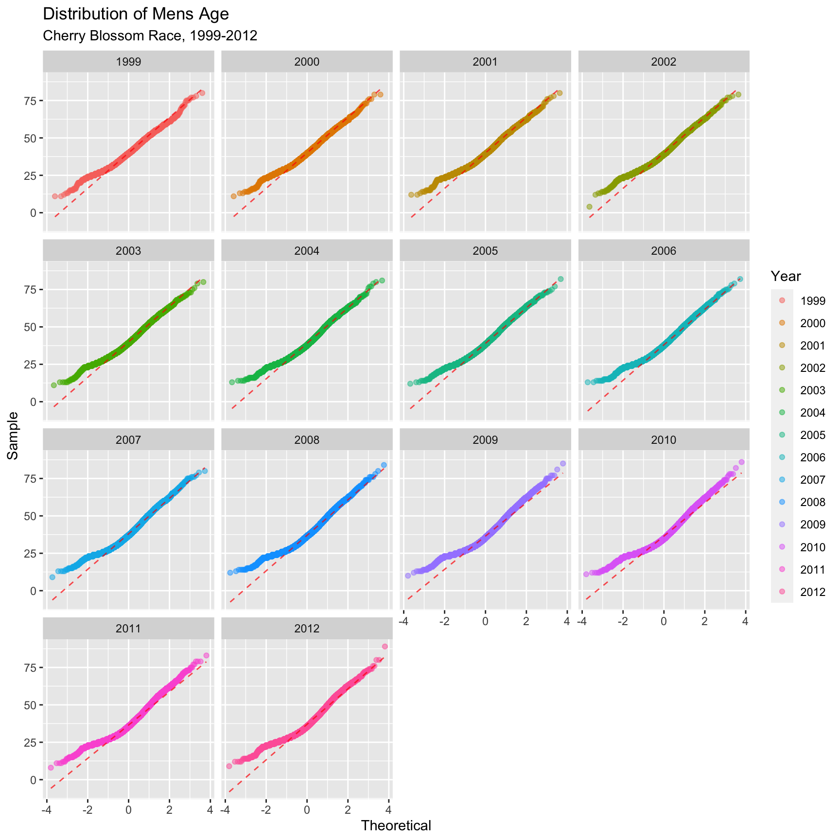
Figure 4.2.1 QQ-plots for mens ages 1999-2012 (CLICK ON PLOT TO ENLARGE)

Animated

Figure 4.2.2 Animated QQ-plots for mens ages 1999-2012 (CLICK ON PLOT TO ENLARGE)

Boxplots

In both Figure 4.3.1 and Figure 4.3.2 below, show boxplots displaying the age of the men entrants for every year. It is very easy to see the shifting mean trend toward younger runners. There is clearly a difference in the mean age between 1999 and 2012, and these plots really display that the shift was gradual from about 40 to 37.

These plots are very useful for showing the yearly movement in the mean age of mens runners, though they fall a little short with truly expressing the yearly differences of the distribution of ages.

All Boxplots

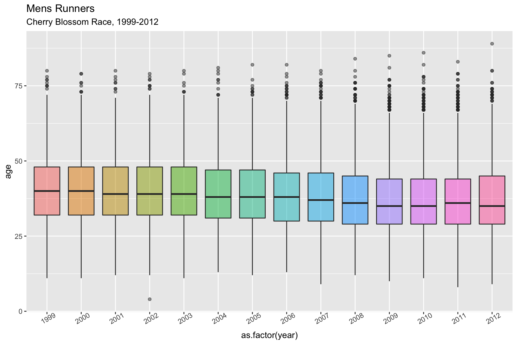
Figure 4.3.1 Boxplots of mens ages 1999-2012 (CLICK ON PLOT TO ENLARGE)

Animated

Figure 4.3.2 Animated Boxplot of mens ages 1999-2012 (CLICK ON PLOT TO ENLARGE)

Density Curves

Figure 4.4.1 and Figure 4.4.2 below, also show the movement in the ages toward a right skewed distribution very well. Figure 4.4.1 with overlaid density curves, the most recent 4 or 5 races show a completely different shape. The majority of racers enrolling in the later years of this range are younger. This is consistent with the movement shown in the QQ-plots and Boxplots above.

The animated Figure 4.4.2 really highlights the shift in the distribution of the racer age is gradual. The curves really start to spike toward the end.

Overlaid

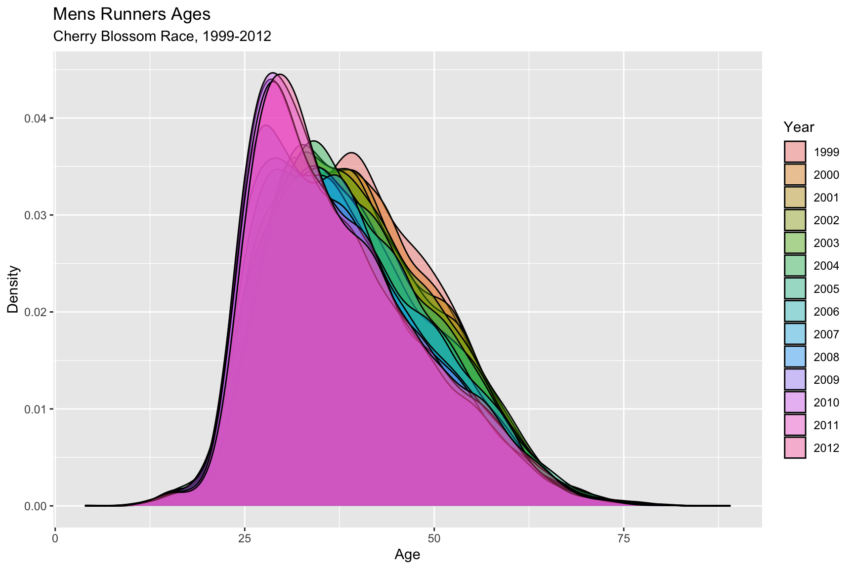
Figure 4.4.1 Overlaid Density Curves, mens ages 1999-2012 (CLICK ON PLOT TO ENLARGE)

Animated

Figure 4.4.2 Animated Distributions of mens ages, 1999-2012 (CLICK ON PLOT TO ENLARGE)

Histograms

Figure 4.5.1 and Figure 4.5.2 below, naturally highlight a similar theme as the density curves of a definitive shift in the age of a majority of the entrants. Figure 4.5.1 shows that in the early years of this range from 1999-2005, there isn’t a big change year over year. Each of these curves have a similar shape with a little, but noticeable growth in the overall total number of annual runners.

Around 2006 there is more noticeable annual growth, particularly with the number of younger racers. This trend continues with for the remainder of years. These figures are very telling about how the distribution is changing. It seems like there are just more younger men entering the races as this range of years progress. This increase in younger runners is quite noticeable, as this increase is certainly the reason for the shift in the mean from 1999-2012.

It appears as though there is annual growth for all age groups, however growth in the younger age groups are more apparent. The next section will expand upon this notion and further examine the yearly growth of the divisions.

Facet Wrapped

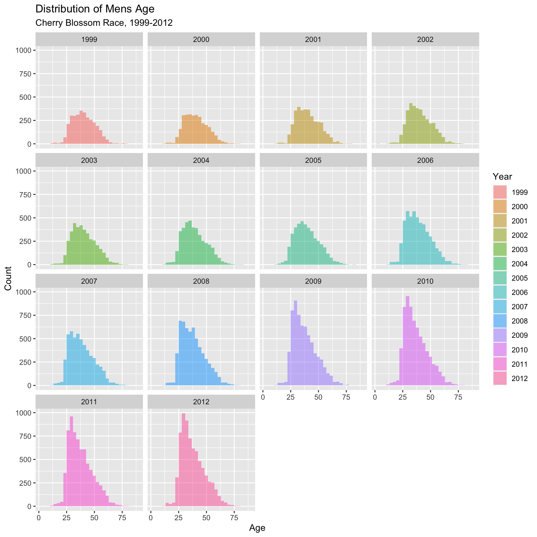
Figure 4.5.1 Histograms for men entrants, 1999-2012 (CLICK ON PLOT TO ENLARGE)

Animated

Figure 4.5.2 Animated Histograms for men entrants, 1999-2012 (CLICK ON PLOT TO ENLARGE)

Annual Growth of Race

The proceeding plots are being displayed to really highlight the annual growth of the race over this range of years in the Mens division. Figure 4.6.1 shows the raw number of competitors, some aspects provide reinforcement what was seen in the histograms. There seems to be a large jump in runners from 2005 to 2006.

Figure 4.6.2 below shows difference in the number of annual competitor from year to year. This was found by taking the first difference with the artrans.wge() function. The increase in number of runners between the years 2005 and 2006 represent the largest increase between any year with large gains in 2008 and 2009 as well.

Figure 4.6.3 shows the increase in competitors at the division level. This really breaks down where the influx of new runners are registering. As expected, the biggest annual increases for the race are coming in the M2529 and M3035, especially in the years identified above as major growth years. These runners are driving the mean age of the male runner down.

Total Number

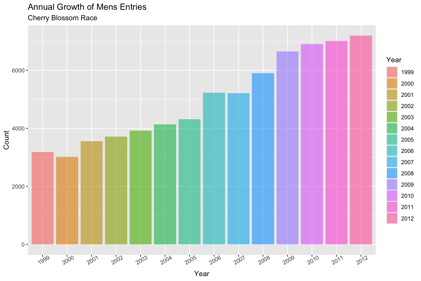
Figure 4.6.1 Number of men runners, 1999-2012 (CLICK ON PLOT TO ENLARGE)

Yearly Change

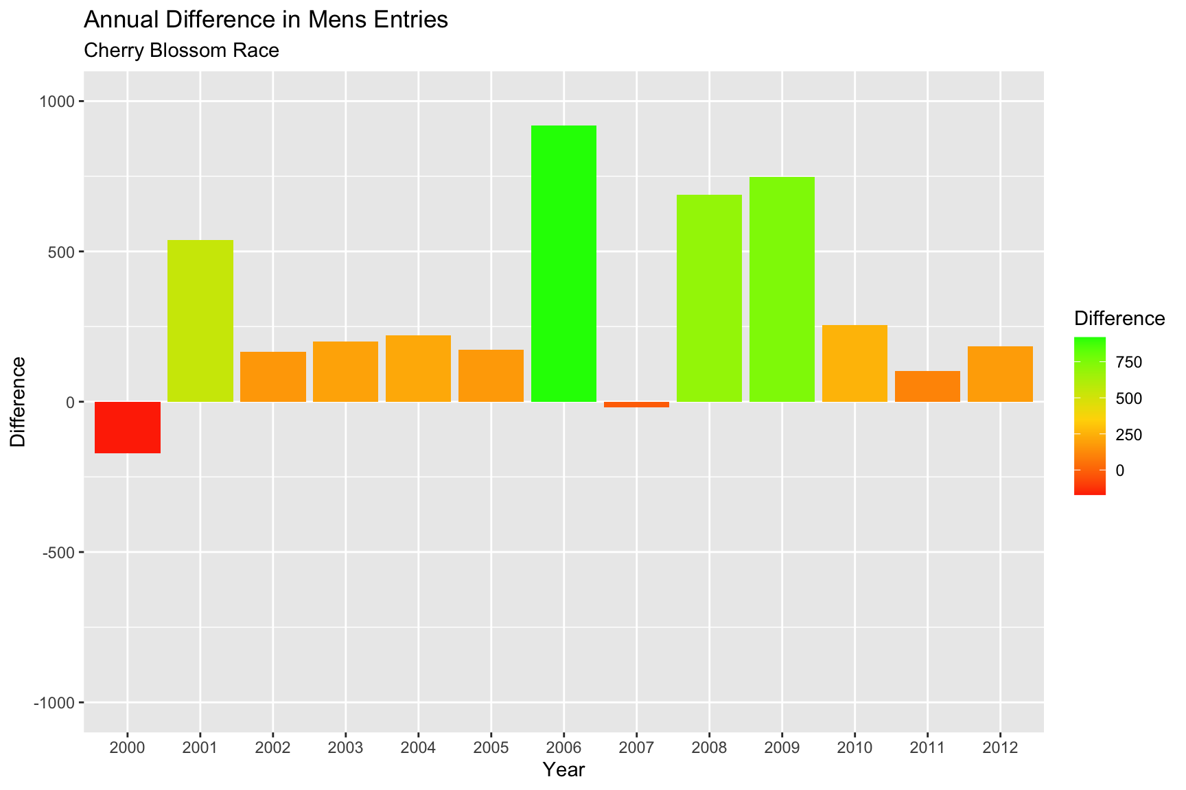
Figure 4.6.2 Yearly difference in total enrollment of men runners, 1999-2012 (CLICK ON PLOT TO ENLARGE)

Yearly Change by Division

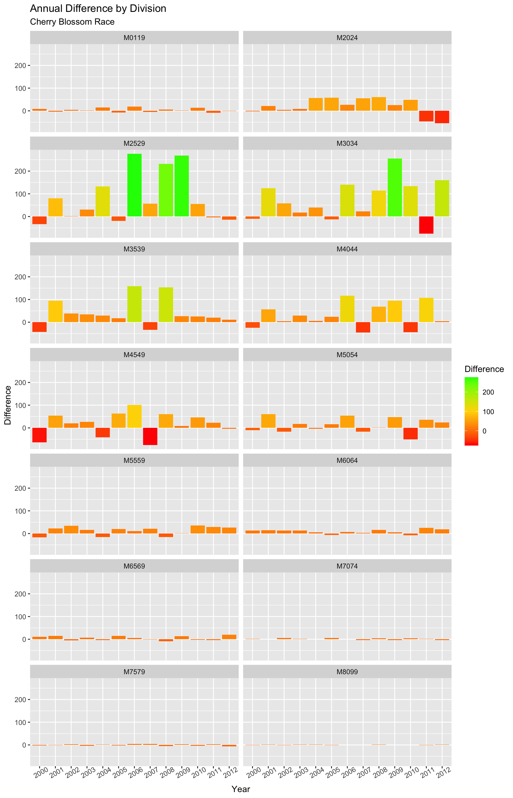
Figure 4.6.3 Yearly difference in divisional enrollment of men runners, 1999-2012 (CLICK ON PLOT TO ENLARGE)

Changepoint Analysis

Figure 5.1 below shows the mean ages of the runners over the course of the years of interest. The last statistical method employed on this dataset was examining the data for possible change points in the mean of the data. The changepoint package was used with two seperate methods of analysis, the “AMOC” or At Most One Change method and Binary segmentation.

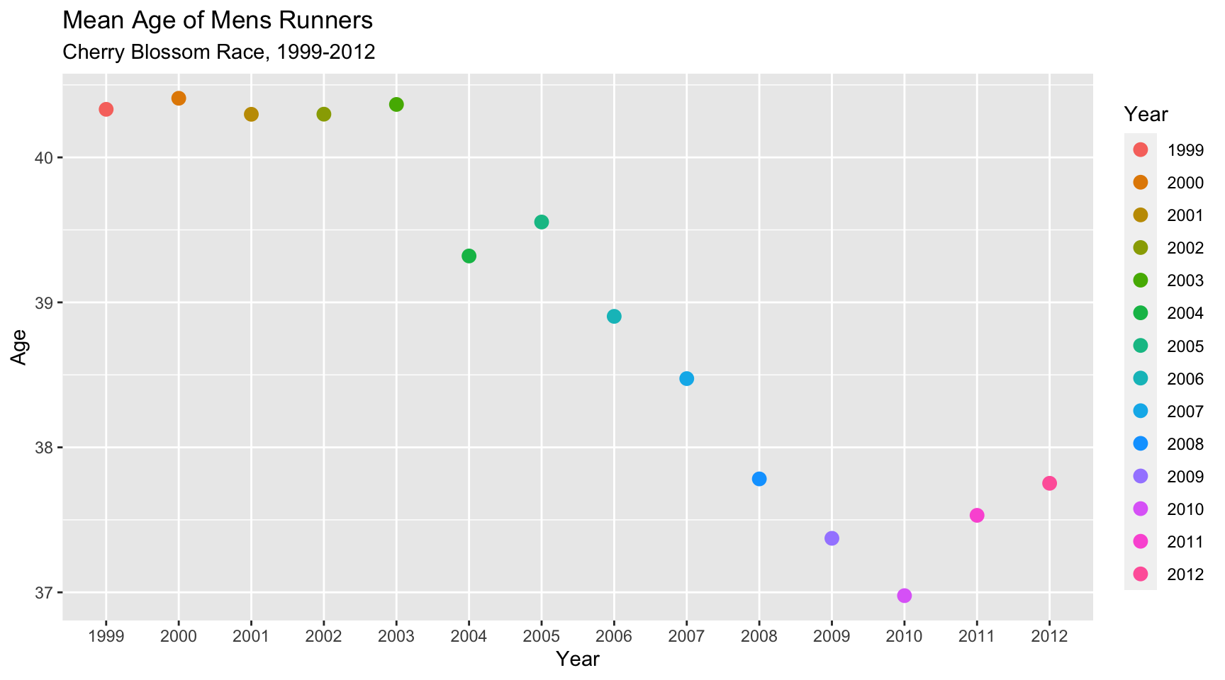
Figure 5.1 Annual Mean in male runners, 1999-2012 (CLICK ON PLOT TO ENLARGE)

Both methods of analysis yielded the same change in mean. Each identified 2006 as the year where the mean in age shifted. This really ties together the trends seen with the plots above, to add some evidence about the data above. The increase in young runners seen between the 2005-2006 had an effect on the mean, which was detected with the changepoint package functions. One cavet is that both function were only to locate 1 changepoint. The binary segmentation method could locate more change points, but if the restrictions are too relaxed, it will identify every change in the data, which isn’t useful.

Summary

There is a very evident shift in the mean ages over this time span, and the shift appears to be gradual. The distribution of the age of men competitors over the course of these years tends to shift more to the right. This shift to a right skew is cause by a large increase in men into the younger divisions and this leads to the mean age being driven down. Changepoint analysis of the time series found there to be a change in the mean age of the competitors to be in 2006, which is the midpoint of the data. Because the midpoint was identified as the change, this would seem to provide evidence that this change was gradual.

What shouldn’t go unnoticed however is that it is a though mean age is shifting younger, this isn’t due to older runners losing interest and not competing in the race. The enrollment for the older runners remains very consistent throughout the entirity of the data set. The cause of the mean shift is due to the large influx of young runners, the reasons for which could be many.

Conclusion

This was another very excellent exercise. The fact that the website had changed made it slightly more of a challenge, but the new website is actually much easier to scrape. It is improved in that each year is in a consistent format. In the asyncronous videos and textbook, there was far more involved with cleaning and formatting the data between the different years. Having an unpredictable annual format is very challenging to automating the scraping process, however this new format seems to alleviated this issue. A draw back is that the process takes longer. Results were only 20 to a page, so roughly 3500 web pages had to be hit to gather just the mens data for this time span, with the original format this number was far less.

Even still with the increased data acquisition time, it was balanced out a bit with less time required for cleaning data. This exercise was a great tool for data collection. Hopefully it is understandable that this case study included both web scraping and analysis. It was quite anticlimactic to invest work in scraping so much data and then not do any type of analysis. Even seeing how this race has changed over time was a very interesting exercise.

Analysis of this data lead to further questions which could be answered if time had permitted additional studies. One topic of interest was to analyze the hometown feature in greater depth. It would be interesting to investigate where the racers are from? Is the annual growth of the race from runners in the US, or has this race attracted the attention of international runners? A function (Further Studies) was created to parse the hometown feature to try to extract this information, however some of the records had difficult formats to create an automated answer. Lastly, naturally the question of the mean age of the women competitors experience a similar change in mean over the same time span? How did this change in mean age effect the mean time of the runners? These are a few further studies which could be conducted on this dataset, along with a host of others.

This was also a great exercise because it showed the duality of web scraping. It is a fantastically powerful way to gather openly available data, but seemingly overnight it can be rendered useless. This case study showed that in the world of data science, one needs to be very flexible and adaptable to different situations, because technology is constantly changing and evolving.

Appendix

Sources

w3schools HTML Tags: https://www.w3schools.com/tags/default.asp

Nolan, Deborah; Lang, Duncan Temple.; Data Science in R: A Case Studies Approach to Computational Reasoning and Problem Solving; Chapter 2 pgs 45-103.

Cherry Blossom Race

Cherry Blossom Race Database

changepoint package

Functions

Fetch Datatable

return_dataTable <- function(url)
{
  # Fetch the page passed as url, expects cherry blossom database site
  # example: http://www.cballtimeresults.org/performances?division=Overall+Women&page=1&section=10M&sex=W&utf8=%E2%9C%93&year=1999
  # Page 1 of Womens 10 Mile from 1999
  page <- xml2::read_html(url)
  
  # create dataframe with results 
  # data needed is in only <table></table> on page, makes it easy
  dataTable <- page %>% # take page
    rvest::html_node("table") %>% # find table
    rvest::html_table() # convert table to dataframe
  
  return(dataTable)
}

The return_dataTable() function puts the data that is in the HTML table on the cherry blossom run database website into a dataframe.

Collect Annual Data

collect_data <- function(year, gender)
{
  # Fetch data for first page of desired gender/year combo, needed to create dataframe to add subsequent pages
  # Column header names created issues with rbind(), got colnames from the site on first page as seed for loop
  # Additionally, this will find out how many pages of results to fetch from the "PiS/TiS" column returned
  url_first <- paste("http://www.cballtimeresults.org/performances?division=Overall+",
                     gender,
                     "&page=",
                     1,
                     "&section=10M&sex=",
                     substring(gender,1,1),
                     "&utf8=%E2%9C%93&year=",
                     year,
                     sep = "")  
  
  # Prints the url of first page to show progress
  print(url_first) 
  
  # Seed dataframe for upcoming loop
  data1 <- return_dataTable(url_first) 
  
  # This column shows Place in Sex/Total in Sex
  n = data1$`PiS/TiS`[1] 
  
  # Split 1st value on / select second element, total runners/gender
  n = as.numeric(strsplit(n,"/")[[1]][2]) 
  
  # Pages display 20 results so this finds the n for pages
  n = trunc(n/20) + 1 
  
  # iterate through pages for the year, adding to seed dataframe per page
  i = 2
  
  for (i in 2:n) {
    url_loop <- paste("http://www.cballtimeresults.org/performances?division=Overall+",
                      gender,
                      "&page=",
                      i,
                      "&section=10M&sex=",
                      substring(gender,1,1),
                      "&utf8=%E2%9C%93&year=",
                      year,
                      sep = "")  
    data2 <- return_dataTable(url_loop)
    print(paste(gender, " - ", i, " - ", year))
    data1 <- bind_rows(mutate_all(data1, as.character), mutate_all(data2, as.character))
  }
    # return entire year df
  return(data1)
}

The collect_data() function will scrape data for a year of data for one gender.

Collect Mutli-Year Data

get_all_data = function(years, gender)
{
  # seed dataframe for loop due to column name issue
  # fetches first year data
  df_all <- collect_data(years[1], gender)
  
  # iterate through the years of single gender passed
  for(i in seq(2, length(years)))
    {
    # add to year of data to total dataframe
    df_all <- bind_rows(
      mutate_all(df_all, as.character), 
      mutate_all(collect_data(years[i],gender), as.character)
      )
  }
  
  # write results to csv with file name "allData[gender].csv" for later analysis
  write_csv(df_all, paste("data/allData", gender,".csv",sep = ""))
  return(df_all)
}

The above function will be passed a list of desired years (1973-present) to retrieve data for a single gender.

Scrape All Data

scrape_data = function()
  {
  # desired years
  years <- seq(1999,2012,1) 
  # Both genders, need to be in this format will be part of url
  genders <- c("Men", "Women")
  for (i in 1:length(genders)) {
    # update print
    print(paste(genders[i], " - Starting"))
    
    # collect all data for both genders
    get_all_data(years, genders[i])
    
    #update print
    print(paste(genders[i], " - COMPLETE!!!"))
  }
  #update print
  print("DATA SCRAPE COMPLETE!!!")
}

The scrape_data function will scrape all the data for men and women for the range of years in this case study.

Data Cleaning Steps

Read Data

# column names for data from site
col_names <- c("race", 
               "name", 
               "age", 
               "time", 
               "pace", 
               "placeInSex", 
               "division", 
               "placeInDivision", 
               "hometown")

# read csv of compiled Mens data
df_all_mens <- read_csv("data/allDataMen.csv", col_types = cols(Age = col_character()))

# set the names for the df
names(df_all_mens) <- col_names

# show how many rows in total dataset
number_of_obs <- dim(df_all_mens)[1]

This block of code will load the mens data.

Formatting

# eliminate rows with NR for age
df_trim <- df_all_mens[which(df_all_mens$age != "NR"),]

# show how many eliminated from data
dim(df_trim)

# switch the age column from character to integer
df_trim$age <- as.integer(df_trim$age)

# this will take the race column split on whitespace, and index year data
minus <- which(unlist(strsplit(df_trim$race, "\\s")) != "10M")

# creates year column 
df_trim$year <- as.integer(unlist(strsplit(df_trim$race, "\\s"))[minus])

# turns division column into factor
df_trim$division <- as.factor(df_trim$division)

This block provides formatting to the mens data frame, outlined in the methods section.

Summary Dataframes

# create summary dataframe by year
df_age_stats <- df_trim %>%
                  group_by(year) %>%
                  summarize(
                    mean = mean(age), 
                    sd = sd(age),
                    oldest = max(age),
                    yngest = min(age),
                    n=n(),
                    skew = skewness(age)
                    )

# create dataframe of number of racers per division, per year
df_div_stats <- df_trim %>%
                  group_by(division, year) %>%
                  summarize(
                    n=n()
                    )

# names for above dataframe, need to add data
div_stat_names <- c("division", "year", "n")

# adding missing data
df_row_to_add <- data.frame("M8099", 2002, 0)
df_row_to_add2 <- data.frame("M8099", 2000, 0)
names(df_row_to_add)<-div_stat_names
names(df_row_to_add2)<-div_stat_names

df_div_stats <- rbind(df_div_stats, df_row_to_add)
df_div_stats <- rbind(df_div_stats, df_row_to_add2)


# !!!!!!! This is where it errors for me !!!!!!!!!

## It worked on my computer...lol, but really maybe it was that chunk I commented out I didn't run it -
## when I went through it, I also didn't have all the right packages in at the top, so I had issues
## making one of the dataframes the first run so maybe that might have been it

# turn divisons into factors
df_div_stats$division <- as.factor(df_div_stats$division)

# order the data correctly chronologically
df_div_stats <- df_div_stats[order(df_div_stats$division, df_div_stats$year),]

The above code chunks produce the summary dataframes which were investigated in the results section.

Changepoint

m.amoc <- cpt.mean(df_age_stats$mean, penalty = "SIC")

cpts(m.amoc)

## [1] 8

m.binseg <- cpt.mean(df_age_stats$mean, method = "BinSeg")

cpts(m.binseg)

## [1] 8

The above chunk finds the change point in the mean age of the men runners over the year range.

Further Studies

extract_state = function(string)
  {
  tmp <- string
  if (grepl(",", string) == "TRUE"){
    tmp <- str_trim(strsplit(string, ",")[[1]][2])
  }
  return(tmp)
}

df_trim$state2 <- unlist(lapply(df_trim$hometown, extract_state))

df_trim$state <- ifelse((grepl(",", df_trim$hometown) == "TRUE"),substr(df_trim$hometown, # nchar(df_trim$hometown) - 2, nchar(df_trim$hometown)), "NaS")

df_trim[which(str_locate(df_trim$hometown, ",") - nchar(df_trim$hometown) != -3),]
df_trim[-which(grepl(",", df_trim$hometown) == "TRUE" | nchar(df_trim$hometown) <= 3),]

unlist(unique(df_trim[-which(grepl(",", df_trim$hometown) == "TRUE" | nchar(df_trim$hometown) <= # 3),"hometown"]))

The hometown feature requires a bit more formatting because it can contain a “city, state” combo for US runners or simply a country for international runners. The next code block splits the hometown field by the comma and when the comma is missing, it is presumed that the runner is international.

For this analysis we are not interested at the state level, but we keep the state and international country data and we put both into a field called “state2”.